Time
For this example, we’re going to use economic data from the US Federal Reserve (the Fed). The St. Louis Fed is in charge of publishing Fed economic data, and they host it all at an online portal named FRED. Instead of downloading individual time series data from the FRED website, we’ll do what with did with the World Bank WDI data and download it directly from the internet with the tidyquant package, which includes a function for working with the FRED API/website.
If you want to skip the data downloading, you can download the data below (you’ll likely need to right click and choose “Save Link As…"):
Live coding example
Complete code
(This is a slightly cleaned up version of the code from the video.)
Get data
First, we load the libraries we’ll be using:
library(tidyverse)  # For ggplot, dplyr, and friends
library(tidyquant)  # For accessing FRED data
library(scales)     # For nicer labels
The US Federal Reserve provides thousands of economic datasets at FRED. We can use the tidyquant R package to access their servers and download the data directly into R.
Like we did with the WDI indicators in session 8, we need to find the special internal code for the variables we want to get. We need to pay close attention to the details of each variable, since the same measure can be offered with different combinations of real (adjusted for inflation) or nominal (not adjusted for inflation); monthly, quarterly, or annually; and seasonally adjusted or not seasonally adjusted. For instance, if you want to see US GDP, here are some possibilities (all the possible GDP measures are listed here):
GDPC1: Real (2012 dollars), quarterly, seasonally adjustedND000334Q: Real (2012 dollars), quarterly, not seasonally adjustedGDPCA: Real (2012 dollars), annual, not seasonally adjustedGDP: Nominal, quarterly, seasonally adjustedGDPA: Nominal, annual, not seasonally adjusted
The code for getting data from FRED works a little differently than WDI(), and the output is a little different too, but it’s hopefully not too complicated. We need to feed the tq_get() function (1) a list of indicators we want, (2) a source for those indicators, and (3) a starting and/or ending date.
tq_get() can actually get data from a ton of different sources like stocks from Yahoo Finance and general financial data from Bloomberg, Quandl, and Tiingo. Most of those other sources require a subscription and a fancy API key that logs you into their servers when getting data, but FRED is free (yay public goods!).
We’ll first make a new dataset named fred_raw that gets a bunch of interesting variables from FRED from January 1, 1990 until today.
fred_raw <- tq_get(c("RSXFSN",  # Advance retail sales
                     "GDPC1",  # GDP
                     "ICSA",  # Initial unemployment claims
                     "FPCPITOTLZGUSA",  # Inflation
                     "UNRATE",  # Unemployment rate
                     "USREC"),  # Recessions
                   get = "economic.data",  # Use FRED
                   from = "1990-01-01")
Downloading data from FRED every time you knit will get tedious and take a long time (plus if their servers are temporarily down, you won’t be able to get the data). As with the World Bank data we used, it’s good practice to save this raw data as a CSV file and then work with that.
write_csv(fred_raw, "data/fred_raw.csv")
Since we care about reproducibility, we still want to include the code we used to get data from FRED, we just don’t want it to actually run. You can include chunks but not run them by setting eval=FALSE in the chunk options. In this little example, we show the code for downloading the data, but we don’t evaluate the chunk. We then include a chunk that loads the data from a CSV file with read_csv(), but we don’t include it (include=FALSE). That way, in the knitted file we see the WDI() code, but in reality it’s loading the data from CSV. Super tricky.
I first download data from FRED:

```{r get-fred-data, eval=FALSE}
fred_raw <- tq_get(...)

write_csv(fred_raw, "data/fred_raw.csv")
```

```{r load-fred-data-real, include=FALSE}
fred_raw <- read_csv("data/fred_raw.csv")
```
Look at and clean data
The data we get from FRED is in a slightly different format than we’re used to with WDI(), but with good reason. With World Bank data, you get data for every country and every year, so there are rows for Afghanistan 2000, Afghanistan 2001, etc. You then get a column for each of the variables you want (population, life expectancy, GDP/capita, etc.)
With FRED data, that kind of format doesn’t work for every possible time series variable because time is spaced differently. If you want to work with annual GDP, you should have a row for each year. If you want quarterly GDP, you should have a row for every quarter. If you put these in the same dataset, you’ll end up with all sorts of missing data issues:
time |
annual_gdp |
quarterly_gdp |
|---|---|---|
| 2019, Q1 | X | X |
| 2019, Q2 | X | |
| 2019, Q3 | X | |
| 2019, Q4 | X | |
| 2020, Q1 | X | X |
| 2020, Q2 | X |
To fix this, the tidyquant package gives you data in tidy (or long) form and only provides three columns:
head(fred_raw)
## # A tibble: 6 × 3
##   symbol date        price
##   <chr>  <date>      <dbl>
## 1 RSXFSN 1992-01-01 130683
## 2 RSXFSN 1992-02-01 131244
## 3 RSXFSN 1992-03-01 142488
## 4 RSXFSN 1992-04-01 147175
## 5 RSXFSN 1992-05-01 152420
## 6 RSXFSN 1992-06-01 151849
The symbol column is the ID of the variable from FRED , date is… the date, and price is the value. These columns are called symbol and price because the tidyquant package was designed to get and process stock data, so you’d typically see stock symbols (like AAPL or MSFT) and stock prices. When working with FRED data, the price column shows the value of whatever you’re interested in—it’s not technically a price (so unemployment claims, inflation rates, and GDP values are still called price).
Right now, our fred_raw dataset has only 3 columns, but nearly 3,000 rows since the six indicators we got from the server are all stacked on top of each other. To actually work with these, we need to filter the raw data so that it only includes the indicators we’re interested in. For instance, if we want to plot retail sales, we need to select only the rows where the symbol is RSXFSN. Make a smaller dataset with filter() to do that:
retail_sales <- fred_raw %>%
  filter(symbol == "RSXFSN")

retail_sales
## # A tibble: 351 × 3
##    symbol date        price
##    <chr>  <date>      <dbl>
##  1 RSXFSN 1992-01-01 130683
##  2 RSXFSN 1992-02-01 131244
##  3 RSXFSN 1992-03-01 142488
##  4 RSXFSN 1992-04-01 147175
##  5 RSXFSN 1992-05-01 152420
##  6 RSXFSN 1992-06-01 151849
##  7 RSXFSN 1992-07-01 152586
##  8 RSXFSN 1992-08-01 152476
##  9 RSXFSN 1992-09-01 148158
## 10 RSXFSN 1992-10-01 155987
## # … with 341 more rows
If multiple variables have the same spacing (annual, quarterly, monthly, weekly), you can use filter to select all of them and then the use pivot_wider() or spread() to make separate columns for each. Inflation, unemployment, and retail sales are all monthly, so we can make a dataset for just those:
fred_monthly_things <- fred_raw %>%
  filter(symbol %in% c("FPCPITOTLZGUSA", "UNRATE", "RSXFSN")) %>%
  # Convert the symbol column into multiple columns, using the "prices" for values
  pivot_wider(names_from = symbol, values_from = price)

fred_monthly_things
## # A tibble: 375 × 4
##    date       RSXFSN FPCPITOTLZGUSA UNRATE
##    <date>      <dbl>          <dbl>  <dbl>
##  1 1992-01-01 130683           3.03    7.3
##  2 1992-02-01 131244          NA       7.4
##  3 1992-03-01 142488          NA       7.4
##  4 1992-04-01 147175          NA       7.4
##  5 1992-05-01 152420          NA       7.6
##  6 1992-06-01 151849          NA       7.8
##  7 1992-07-01 152586          NA       7.7
##  8 1992-08-01 152476          NA       7.6
##  9 1992-09-01 148158          NA       7.6
## 10 1992-10-01 155987          NA       7.3
## # … with 365 more rows
But wait! There’s a problem! The inflation rate we got isn’t actually monthly—it seems to be annual, which explains all the NAs. Let’s fix it by not including it. We’ll also rename the columns so they’re easier to work with
fred_monthly_things <- fred_raw %>%
  filter(symbol %in% c("UNRATE", "RSXFSN")) %>%
  # Convert the symbol column into multiple columns, using the "prices" for values
  pivot_wider(names_from = symbol, values_from = price) %>%
  rename(unemployment = UNRATE, retail_sales = RSXFSN)

fred_monthly_things
## # A tibble: 375 × 3
##    date       retail_sales unemployment
##    <date>            <dbl>        <dbl>
##  1 1992-01-01       130683          7.3
##  2 1992-02-01       131244          7.4
##  3 1992-03-01       142488          7.4
##  4 1992-04-01       147175          7.4
##  5 1992-05-01       152420          7.6
##  6 1992-06-01       151849          7.8
##  7 1992-07-01       152586          7.7
##  8 1992-08-01       152476          7.6
##  9 1992-09-01       148158          7.6
## 10 1992-10-01       155987          7.3
## # … with 365 more rows
All better.
We can make as many subsets of the long, tidy, raw data as we want.
Plotting time
Let’s plot some of these and see what the trends look like. We’ll just use geom_line().
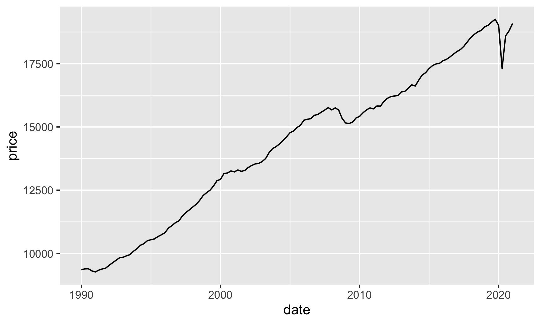
Here’s GDP:
# Get just GDP data from the raw FRED data
gdp_only <- fred_raw %>%
  filter(symbol == "GDPC1")

ggplot(gdp_only, aes(x = date, y = price)) +
  geom_line()
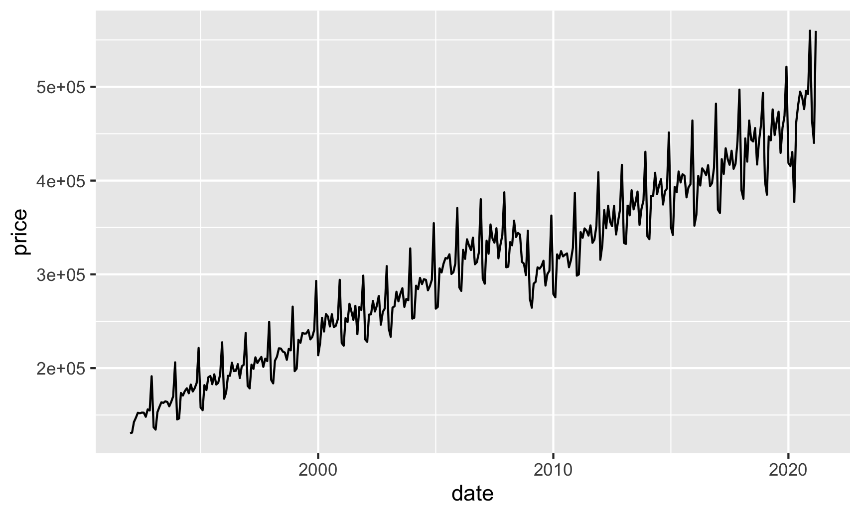
Here’s retail sales:
# Get just GDP data from the raw FRED data
retail_sales_only <- fred_raw %>%
  filter(symbol == "RSXFSN")

ggplot(retail_sales_only, aes(x = date, y = price)) +
  geom_line()
And here’s unemployment claims:
unemployment_claims_only <- fred_raw %>%
  filter(symbol == "ICSA")

ggplot(unemployment_claims_only, aes(x = date, y = price)) +
  geom_line()
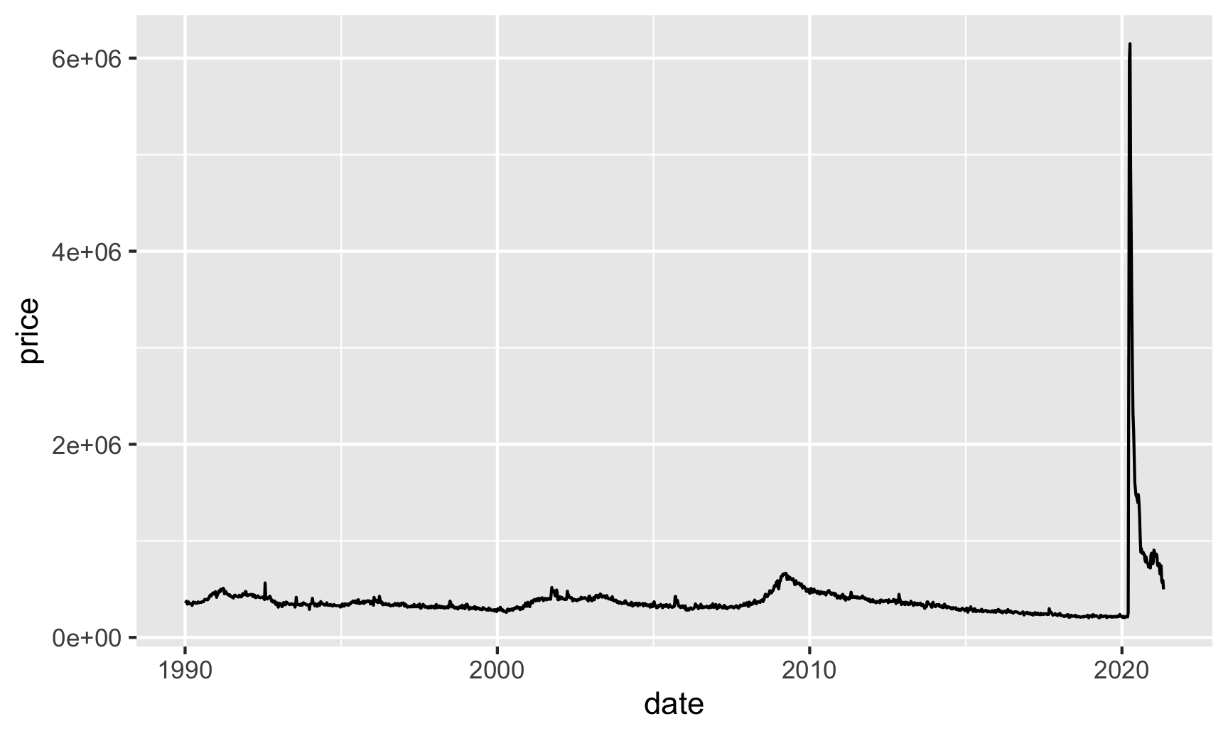
Yikes COVID-19.
There, we visualized time. ✅
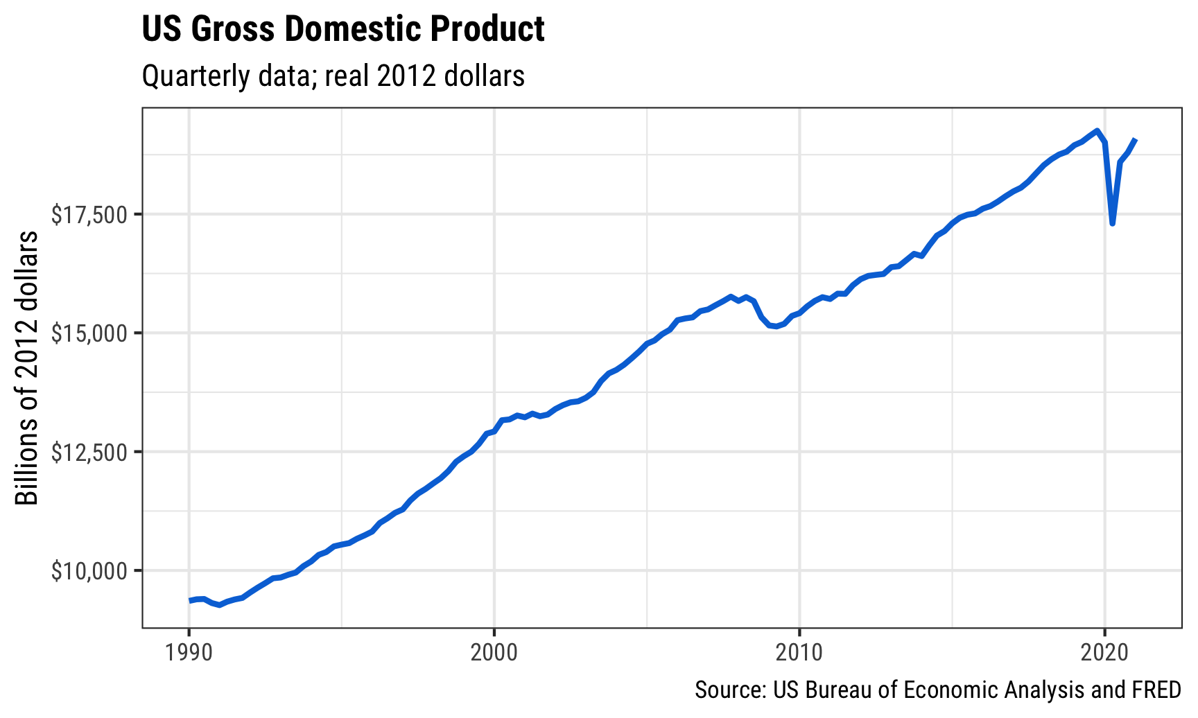
Improving graphics
These were simple graphs and they’re kind of helpful, but they’re not incredibly informative. We can clean these up a little. First we can change the labels and themes and colors:
ggplot(gdp_only, aes(x = date, y = price)) +
  geom_line(color = "#0074D9", size = 1) +
  scale_y_continuous(labels = dollar) +
  labs(y = "Billions of 2012 dollars",
       x = NULL,
       title = "US Gross Domestic Product",
       subtitle = "Quarterly data; real 2012 dollars",
       caption = "Source: US Bureau of Economic Analysis and FRED") +
  theme_bw(base_family = "Roboto Condensed") +
  theme(plot.title = element_text(face = "bold"))
That’s great and almost good enough to publish! We can add one additional layer of information onto the plot and highlight when recessions start and end. We included a recessions variable (USREC) when we got data from FRED, so let’s see what it looks like:
fred_raw %>%
  filter(symbol == "USREC")
## # A tibble: 375 × 3
##    symbol date       price
##    <chr>  <date>     <dbl>
##  1 USREC  1990-01-01     0
##  2 USREC  1990-02-01     0
##  3 USREC  1990-03-01     0
##  4 USREC  1990-04-01     0
##  5 USREC  1990-05-01     0
##  6 USREC  1990-06-01     0
##  7 USREC  1990-07-01     0
##  8 USREC  1990-08-01     1
##  9 USREC  1990-09-01     1
## 10 USREC  1990-10-01     1
## # … with 365 more rows
This is monthly data that shows a 1 if we were in a recession that month and a 0 if we weren’t. The Fed doesn’t decide when recessions happen—the National Bureau of Economic Research (NBER) does, and they have specific guidelines for defining one. We’re probably in one right now, but there’s not enough data for NBER to formally declare it yet.
This data is long and tidy, but that makes it harder to work with given our GDP. We want the start and end dates for each recession so that we can shade those areas on the plot. To find those dates, we need to do a little data reshaping. First, we’ll create a temporary variable that marks if there was a switch from 0 to 1 or 1 to 0 in a given row by looking at the previous row
recessions_tidy <- fred_raw %>%
  filter(symbol == "USREC") %>%
  mutate(recession_change = price - lag(price))
recessions_tidy
## # A tibble: 375 × 4
##    symbol date       price recession_change
##    <chr>  <date>     <dbl>            <dbl>
##  1 USREC  1990-01-01     0               NA
##  2 USREC  1990-02-01     0                0
##  3 USREC  1990-03-01     0                0
##  4 USREC  1990-04-01     0                0
##  5 USREC  1990-05-01     0                0
##  6 USREC  1990-06-01     0                0
##  7 USREC  1990-07-01     0                0
##  8 USREC  1990-08-01     1                1
##  9 USREC  1990-09-01     1                0
## 10 USREC  1990-10-01     1                0
## # … with 365 more rows
Notice the new column we have that is mostly 0s, but 1 when there’s a switch, like in August 1990. 1 means we went from 0 to 1 (no recession → recession), while -1 means we went from 1 to 0 (recession → no recession).
We can see all the start and end dates if we filter:
recessions_start_end <- fred_raw %>%
  filter(symbol == "USREC") %>%
  mutate(recession_change = price - lag(price)) %>%
  filter(recession_change != 0)
recessions_start_end
## # A tibble: 7 × 4
##   symbol date       price recession_change
##   <chr>  <date>     <dbl>            <dbl>
## 1 USREC  1990-08-01     1                1
## 2 USREC  1991-04-01     0               -1
## 3 USREC  2001-04-01     1                1
## 4 USREC  2001-12-01     0               -1
## 5 USREC  2008-01-01     1                1
## 6 USREC  2009-07-01     0               -1
## 7 USREC  2020-03-01     1                1
Finally, we can use tibble() to create a brand new little dataset that includes columns for the start and end dates. Since we’re currently in a recession, we have a little bit of a problem—there’s no end date to the current recession, so we can’t plot it. We need to create our own fake end date for the sake of putting it on a graph. We’ll add a row to recessions_start_end using bind_rows() and give it today’s date with today() (today() by itself returns regular text like "2022-06-01"; we need to tell R that this is a date by feeding it to ymd()).
We can then extract the pairs of recession start and end dates in a miniature dataset of recessions.
# If you're running this code not during a recession, there's no need for this
# intermediate step
recessions_fake_end <- recessions_start_end %>%
  bind_rows(tibble(date = ymd(today()),
                   recession_change = -1))

recessions <- tibble(start = filter(recessions_fake_end, recession_change == 1)$date,
                     end = filter(recessions_fake_end, recession_change == -1)$date)
recessions
## # A tibble: 4 × 2
##   start      end
##   <date>     <date>
## 1 1990-08-01 1991-04-01
## 2 2001-04-01 2001-12-01
## 3 2008-01-01 2009-07-01
## 4 2020-03-01 2022-05-31
We can now add this tiny dataset to our plot using geom_rect(). Notice how we put geom_rect() before geom_line()—that’s so the recession rectangles go under the line instead of on top of it. Also notice that we have to specify 4 new aesthetics for geom_rect(): min and max values for both x and y. We use the recession start and end dates for xmin and xmax, and then use −∞ and ∞ for ymin and ymax to make the rectangles stretch from the bottom of the plot to the top.
The last odd/new thing here is that we also use inherit.aes = FALSE in geom_rect(). That’s because we specified a global x and y aesthetic in ggplot(), which applies to all the other layers we add. geom_rect() doesn’t use x or y, though, and it’ll complain that those columns are missing. The inherit.aes argument tells ggplot that the geom_rect() layer should not get any of the global aesthetics like x or y.
ggplot(gdp_only, aes(x = date, y = price)) +
  geom_rect(data = recessions,
            aes(xmin = start, xmax = end, ymin = -Inf, ymax = Inf),
            inherit.aes = FALSE, fill = "#B10DC9", alpha = 0.3) +
  geom_line(color = "#0074D9", size = 1) +
  scale_y_continuous(labels = dollar) +
  labs(y = "Billions of 2012 dollars",
       x = NULL,
       title = "US Gross Domestic Product",
       subtitle = "Quarterly data; real 2012 dollars",
       caption = "Source: US Bureau of Economic Analysis and FRED") +
  theme_bw(base_family = "Roboto Condensed") +
  theme(plot.title = element_text(face = "bold"))
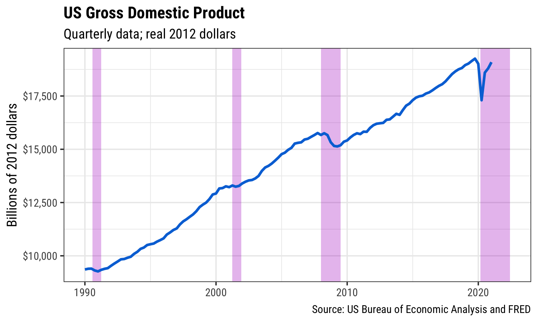
And that’s it!
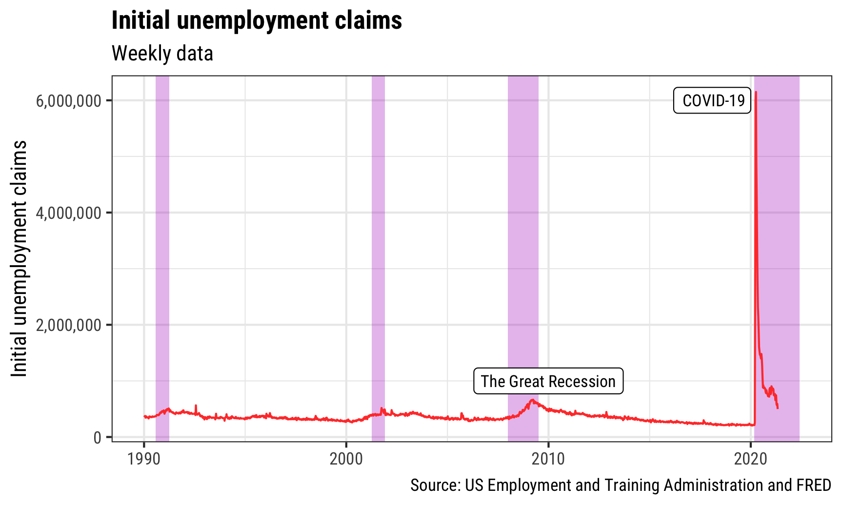
Now that we have the tiny recessions data frame, we can add it to any plot we want. Here’s initial unemployment claims with some extra annotations for fun:
ggplot(unemployment_claims_only, aes(x = date, y = price)) +
  geom_rect(data = recessions,
            aes(xmin = start, xmax = end, ymin = -Inf, ymax = Inf),
            inherit.aes = FALSE, fill = "#B10DC9", alpha = 0.3) +
  geom_line(color = "#FF4136", size = 0.5) +
  annotate(geom = "label", x = as.Date("2010-01-01"), y = 1000000,
           label = "The Great Recession", size = 3, family = "Roboto Condensed") +
  annotate(geom = "label", x = as.Date("2020-01-01"), y = 6000000,
           label = "COVID-19", size = 3, family = "Roboto Condensed", hjust = 1) +
  scale_y_continuous(labels = comma) +
  labs(y = "Initial unemployment claims",
       x = NULL,
       title = "Initial unemployment claims",
       subtitle = "Weekly data",
       caption = "Source: US Employment and Training Administration and FRED") +
  theme_bw(base_family = "Roboto Condensed") +
  theme(plot.title = element_text(face = "bold"))
Decomposition
The mechanics of decomposing and forecasting time series goes beyond the scope of this class, but there are lots of resources you can use to learn more, including this phenomenal free textbook.
There’s a whole ecosystem of time-related packages that make working with time and decomposing trends easy (named tidyverts):
- lubridate: Helpful functions for manipulating dates (you’ve used this before)
- tsibble: Add fancy support for time variables to data frames
- feasts: Decompose time series and do other statistical things with time
- fable: Make forecasts
Here’s a super short example of how these all work.
The retail sales data we got from FRED was not seasonally adjusted, so it looks like it has a heartbeat embedded in it:
retail_sales <- fred_raw %>%
  filter(symbol == "RSXFSN")

ggplot(retail_sales, aes(x = date, y = price)) +
  geom_line()

We can divide this trend into its main components: the trend, the seasonality, and stuff that’s not explained by either the trend or the seasonality. To do that, we need to first modify our little dataset and tell it to be a time-enabled data frame (a tsibble) that is indexed by the year+month for each row. We’ll create a new column called year_month and then use as_tsibble() to tell R that this is really truly dealing with time:
library(tsibble)  # For embedding time things into data frames

retail_sales <- fred_raw %>%
  filter(symbol == "RSXFSN") %>%
  mutate(year_month = yearmonth(date)) %>%
  as_tsibble(index = year_month)
retail_sales
## # A tsibble: 351 x 4 [1M]
##    symbol date        price year_month
##    <chr>  <date>      <dbl>      <mth>
##  1 RSXFSN 1992-01-01 130683   1992 Jan
##  2 RSXFSN 1992-02-01 131244   1992 Feb
##  3 RSXFSN 1992-03-01 142488   1992 Mar
##  4 RSXFSN 1992-04-01 147175   1992 Apr
##  5 RSXFSN 1992-05-01 152420   1992 May
##  6 RSXFSN 1992-06-01 151849   1992 Jun
##  7 RSXFSN 1992-07-01 152586   1992 Jul
##  8 RSXFSN 1992-08-01 152476   1992 Aug
##  9 RSXFSN 1992-09-01 148158   1992 Sep
## 10 RSXFSN 1992-10-01 155987   1992 Oct
## # … with 341 more rows
Notice that the year_month column is now just the year+month. Neato.
Next we need to create a time series model using that data. There are lots of different ways to model time series, and distinguishing between the different types is way beyond the scope of this class. Rob Hyndman’s free books covers them all. We’ll do this with STL decomposition ("Seasonal and Trend decomposition using Loess”) There are other models we can use, like ETS or ARIMA, but again, that’s all beyond this class.
library(feasts)  # For decomposition things like STL()

retail_model <- retail_sales %>%
  model(stl = STL(price))
retail_model
## # A mable: 1 x 1
##       stl
##   <model>
## 1   <STL>
The decomposition model we create is kind of boring and useless—it’s all stored in a single cell.
We can extract the different components of the decomposition with the components() function:
retail_components <- components(retail_model)
retail_components
## # A dable: 351 x 7 [1M]
## # Key:     .model [1]
## # :        price = trend + season_year + remainder
##    .model year_month  price   trend season_year remainder season_adjust
##    <chr>       <mth>  <dbl>   <dbl>       <dbl>     <dbl>         <dbl>
##  1 stl      1992 Jan 130683 148390.     -21901.    4195.        152584.
##  2 stl      1992 Feb 131244 148904.     -22686.    5026.        153930.
##  3 stl      1992 Mar 142488 149418.      -1804.   -5126.        144292.
##  4 stl      1992 Apr 147175 149932.      -2815.      57.9       149990.
##  5 stl      1992 May 152420 150478.       5337.   -3394.        147083.
##  6 stl      1992 Jun 151849 151023.       3011.   -2185.        148838.
##  7 stl      1992 Jul 152586 151569.        350.     667.        152236.
##  8 stl      1992 Aug 152476 152145.       3967.   -3635.        148509.
##  9 stl      1992 Sep 148158 152720.      -5497.     935.        153655.
## 10 stl      1992 Oct 155987 153296.        116.    2575.        155871.
## # … with 341 more rows
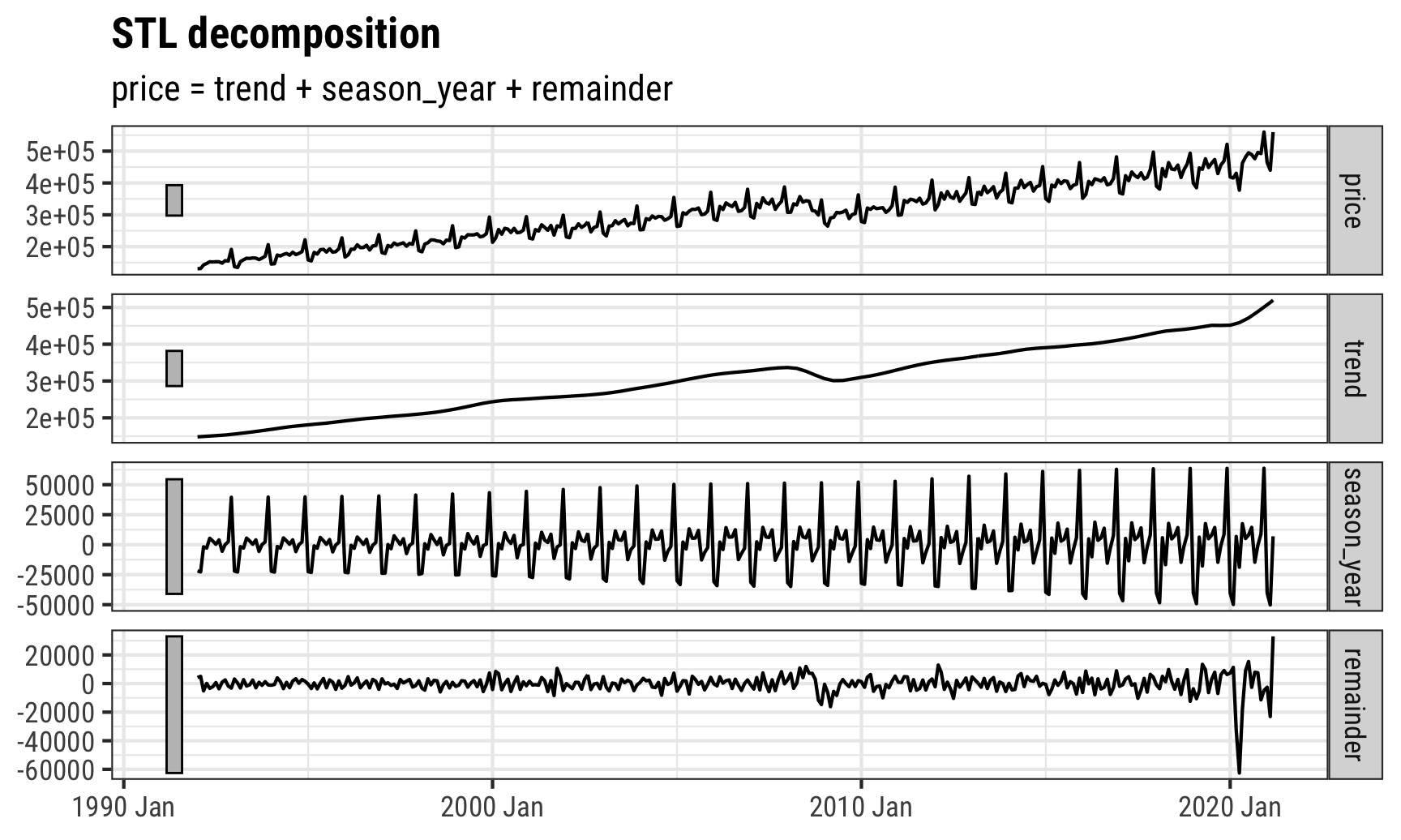
And we can use the autoplot() function from the feasts package to quickly plot all the components. The plot that autoplot() creates is made with ggplot, so any normal ggplot layers work with it:
autoplot(retail_components) +
  labs(x = NULL) +
  theme_bw(base_family = "Roboto Condensed") +
  theme(plot.title = element_text(face = "bold"))
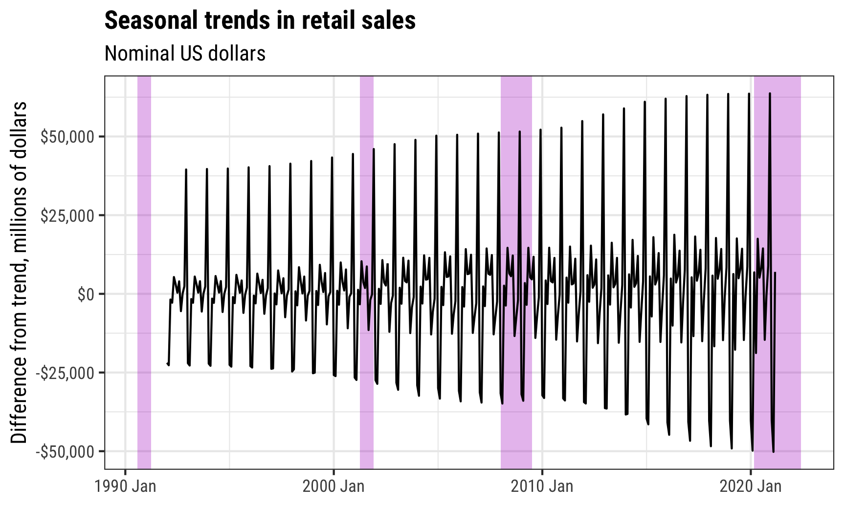
We can also plot individual components on their own using the retail_components dataset we made. Here’s seasonality by itself:
ggplot(retail_components,
       aes(x = year_month, y = season_year)) +
  geom_rect(data = recessions,
            aes(xmin = start, xmax = end, ymin = -Inf, ymax = Inf),
            inherit.aes = FALSE, fill = "#B10DC9", alpha = 0.3) +
  geom_line() +
  scale_y_continuous(labels = dollar) +
  # ggplot needs to know that the main data is a yearmonth column so that it'll
  # deal with the recessions data correctly; without this, you'll get an error
  scale_x_yearmonth() +
  labs(x = NULL, y = "Difference from trend, millions of dollars",
       title = "Seasonal trends in retail sales",
       subtitle = "Nominal US dollars") +
  theme_bw(base_family = "Roboto Condensed") +
  theme(plot.title = element_text(face = "bold"))
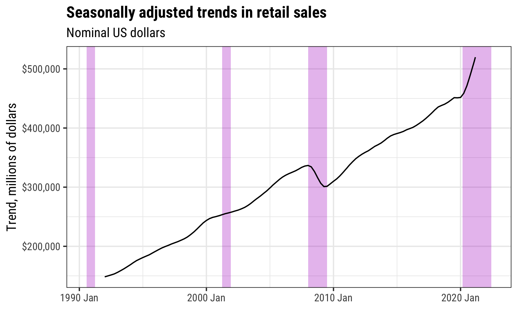
And here’s the trend by itself:
ggplot(retail_components,
       aes(x = year_month, y = trend)) +
  geom_rect(data = recessions,
            aes(xmin = start, xmax = end, ymin = -Inf, ymax = Inf),
            inherit.aes = FALSE, fill = "#B10DC9", alpha = 0.3) +
  geom_line() +
  scale_y_continuous(labels = dollar) +
  scale_x_yearmonth() +
  labs(x = NULL, y = "Trend, millions of dollars",
       title = "Seasonally adjusted trends in retail sales",
       subtitle = "Nominal US dollars") +
  theme_bw(base_family = "Roboto Condensed") +
  theme(plot.title = element_text(face = "bold"))
If you want more control over the combined decomposed plot you can either (1) make individual plots for each of the components and then stitch them together with patchwork, or (2) make the components dataset tidy and facet by component. Here’s what that looks like:
retail_components_tidy <- retail_components %>%
  # Get rid of this column
  select(-season_adjust) %>%
  # Take all these component columns and put them into a long column
  pivot_longer(cols = c(price, trend, season_year, remainder),
               names_to = "component", values_to = "value") %>%
  # Recode this values so they're nicer
  mutate(component = recode(component,
                            price = "Actual data",
                            trend = "Trend",
                            season_year = "Seasonality",
                            remainder = "Remainder")) %>%
  # Make the component categories follow the order they're in in the data so
  # that "Actual data" is first, etc.
  mutate(component = fct_inorder(component))

retail_components_tidy
## # A tsibble: 1,404 x 4 [1M]
## # Key:       .model, component [4]
##    .model year_month component     value
##    <chr>       <mth> <fct>         <dbl>
##  1 stl      1992 Jan Actual data 130683
##  2 stl      1992 Jan Trend       148390.
##  3 stl      1992 Jan Seasonality -21901.
##  4 stl      1992 Jan Remainder     4195.
##  5 stl      1992 Feb Actual data 131244
##  6 stl      1992 Feb Trend       148904.
##  7 stl      1992 Feb Seasonality -22686.
##  8 stl      1992 Feb Remainder     5026.
##  9 stl      1992 Mar Actual data 142488
## 10 stl      1992 Mar Trend       149418.
## # … with 1,394 more rows
Now that we have a long dataset, we can facet by component:
ggplot(retail_components_tidy,
       aes(x = year_month, y = value)) +
  geom_rect(data = recessions,
            aes(xmin = start, xmax = end, ymin = -Inf, ymax = Inf),
            inherit.aes = FALSE, fill = "#B10DC9", alpha = 0.3) +
  geom_line() +
  scale_y_continuous(labels = dollar) +
  scale_x_yearmonth() +
  labs(x = NULL, y = "Millions of dollars",
       title = "Decomposed US Advance Retail Sales",
       subtitle = "Nominal US dollars",
       caption = "Source: US Census Bureau and FRED (RSXFSN)") +
  facet_wrap(vars(component), ncol = 1, scales = "free_y") +
  theme_minimal(base_family = "Roboto Condensed") +
  theme(plot.title = element_text(face = "bold"),
        plot.title.position = "plot",
        strip.text = element_text(face = "bold", hjust = 0))
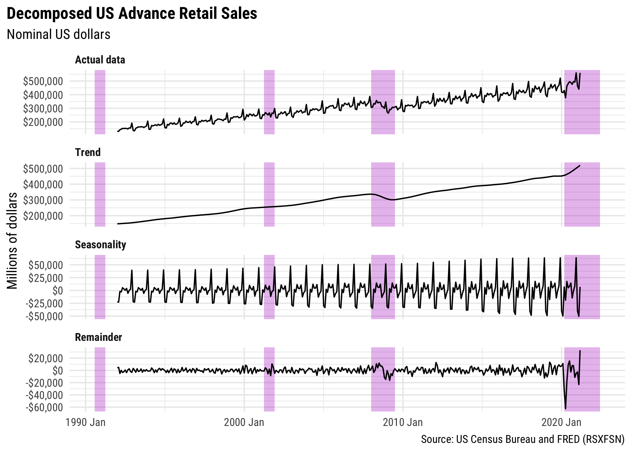
Beautiful!