Comparisons
For this example, we’re going to use cross-national data, but instead of using the typical gapminder dataset, we’re going to collect data directly from the World Bank’s Open Data portal
If you want to skip the data downloading, you can download the data below (you’ll likely need to right click and choose “Save Link As…"):
Live coding example
Complete code
(This is a slightly cleaned up version of the code from the video.)
Load and clean data
First, we load the libraries we’ll be using:
library(tidyverse)  # For ggplot, dplyr, and friends
library(WDI)        # For getting data from the World Bank
library(geofacet)   # For map-shaped facets
library(scales)     # For helpful scale functions like dollar()
library(ggrepel)    # For non-overlapping labels
The World Bank has a ton of country-level data at data.worldbank.org. We can use a package named WDI (world development indicators) to access their servers and download the data directly into R.
To do this, we need to find the special World Bank codes for specific variables we want to get. These codes come from the URLs of the World Bank’s website. For instance, if you search for “access to electricity” at the World Bank’s website, you’ll find this page. If you look at the end of the URL, you’ll see a cryptic code: EG.ELC.ACCS.ZS. That’s the World Bank’s ID code for the “Access to electricity (% of population)” indicator.
We can feed a list of ID codes to the WDI() function to download data for those specific indicators. We want data from 1995-2015, so we set the start and end years accordingly. The extra=TRUE argument means that it’ll also include other helpful details like region, aid status, etc. Without it, it would only download the indicators we listed.
indicators <- c("SP.DYN.LE00.IN",  # Life expectancy
                "EG.ELC.ACCS.ZS",  # Access to electricity
                "EN.ATM.CO2E.PC",  # CO2 emissions
                "NY.GDP.PCAP.KD")  # GDP per capita

wdi_raw <- WDI(country = "all", indicators, extra = TRUE,
               start = 1995, end = 2015)

head(wdi_raw)
Downloading data from the World Bank every time you knit will get tedious and take a long time (plus if their servers are temporarily down, you won’t be able to get the data). It’s good practice to save this raw data as a CSV file and then work with that.
write_csv(wdi_raw, "data/wdi_raw.csv")
Since we care about reproducibility, we still want to include the code we used to get data from the World Bank, we just don’t want it to actually run. You can include chunks but not run them by setting eval=FALSE in the chunk options. In this little example, we show the code for downloading the data, but we don’t evaluate the chunk. We then include a chunk that loads the data from a CSV file with read_csv(), but we don’t include it (include=FALSE). That way, in the knitted file we see the WDI() code, but in reality it’s loading the data from CSV. Super tricky.
I first download data from the World Bank:

```{r get-wdi-data, eval=FALSE}
wdi_raw <- WDI(...)

write_csv(wdi_raw, "data/wdi_raw.csv")
```

```{r load-wdi-data-real, include=FALSE}
wdi_raw <- read_csv("data/wdi_raw.csv")
```
Then we clean up the data a little, filtering out rows that aren’t actually countries and renaming the ugly World Bank code columns to actual words:
wdi_clean <- wdi_raw %>%
  filter(region != "Aggregates") %>%
  select(iso2c, country, year,
         life_expectancy = SP.DYN.LE00.IN,
         access_to_electricity = EG.ELC.ACCS.ZS,
         co2_emissions = EN.ATM.CO2E.PC,
         gdp_per_cap = NY.GDP.PCAP.KD,
         region, income)

head(wdi_clean)
## # A tibble: 6 × 9
##   iso2c country  year life_expectancy access_to_electricity co2_emissions gdp_per_cap region                income
##   <chr> <chr>   <dbl>           <dbl>                 <dbl>         <dbl>       <dbl> <chr>                 <chr>
## 1 AD    Andorra  2015              NA                   100         NA         41768. Europe & Central Asia High income
## 2 AD    Andorra  2004              NA                   100          7.36      47033. Europe & Central Asia High income
## 3 AD    Andorra  2001              NA                   100          7.79      41421. Europe & Central Asia High income
## 4 AD    Andorra  2002              NA                   100          7.59      42396. Europe & Central Asia High income
## 5 AD    Andorra  2014              NA                   100          5.83      40790. Europe & Central Asia High income
## 6 AD    Andorra  1995              NA                   100          6.66      32918. Europe & Central Asia High income
Small multiples
First we can make some small multiples plots and show life expectancy over time for a handful of countries. We’ll make a list of some countries chosen at random while I scrolled through the data, and then filter our data to include only those rows. We then plot life expectancy, faceting by country.
life_expectancy_small <- wdi_clean %>%
  filter(country %in% c("Argentina", "Bolivia", "Brazil",
                        "Belize", "Canada", "Chile"))

ggplot(data = life_expectancy_small,
       mapping = aes(x = year, y = life_expectancy)) +
  geom_line(size = 1) +
  facet_wrap(vars(country))
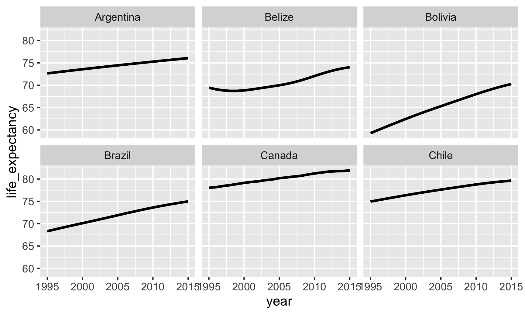
Small multiples! That’s all we need to do.
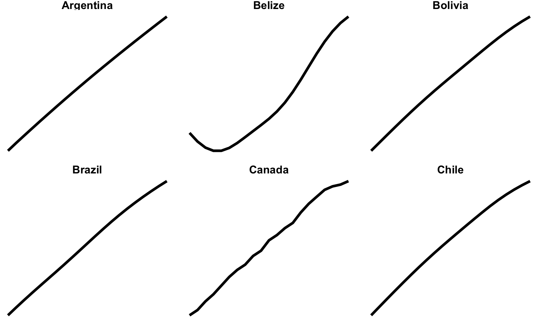
We can do some fancier things, though. We can make this plot hyper minimalist:
ggplot(data = life_expectancy_small,
       mapping = aes(x = year, y = life_expectancy)) +
  geom_line(size = 1) +
  facet_wrap(vars(country), scales = "free_y") +
  theme_void() +
  theme(strip.text = element_text(face = "bold"))
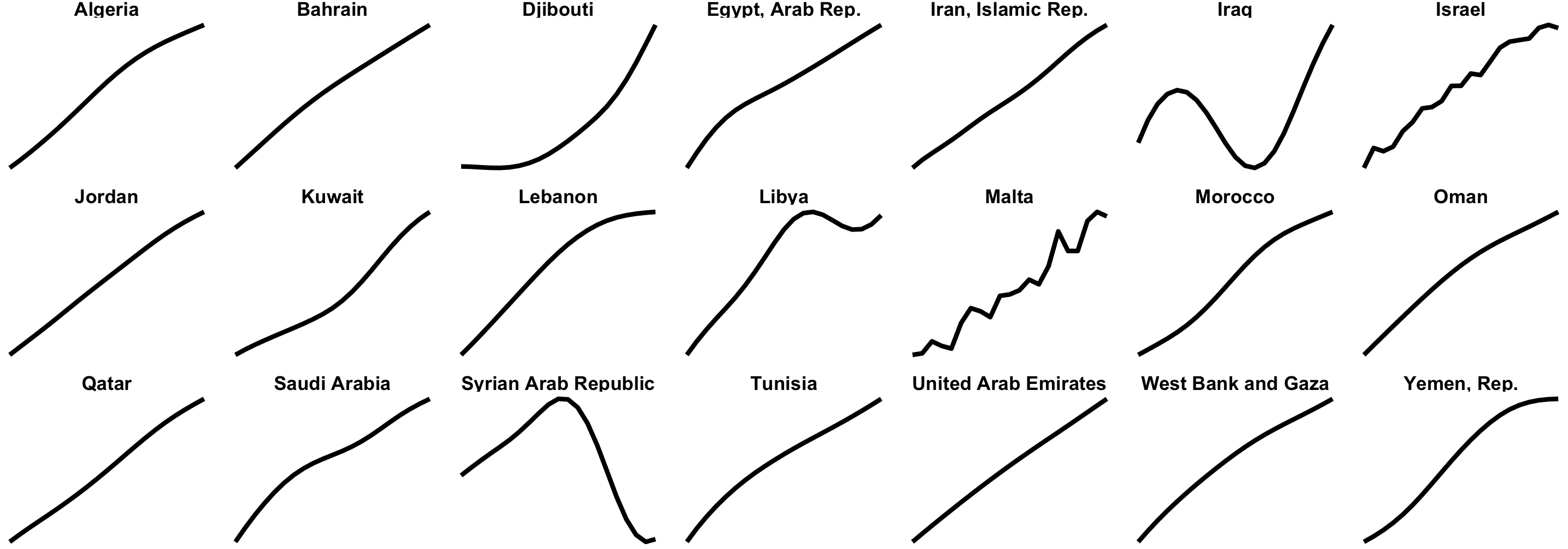
We can do a whole part of a continent (poor Iraq and Syria 😭)
life_expectancy_mena <- wdi_clean %>%
  filter(region == "Middle East & North Africa")

ggplot(data = life_expectancy_mena,
       mapping = aes(x = year, y = life_expectancy)) +
  geom_line(size = 1) +
  facet_wrap(vars(country), scales = "free_y", nrow = 3) +
  theme_void() +
  theme(strip.text = element_text(face = "bold"))
We can use the geofacet package to arrange these facets by geography:
life_expectancy_eu <- wdi_clean %>%
  filter(region == "Europe & Central Asia")

ggplot(life_expectancy_eu, aes(x = year, y = life_expectancy)) +
  geom_line(size = 1) +
  facet_geo(vars(country), grid = "eu_grid1", scales = "free_y") +
  labs(x = NULL, y = NULL, title = "Life expectancy from 1995–2015",
       caption = "Source: The World Bank (SP.DYN.LE00.IN)") +
  theme_minimal() +
  theme(strip.text = element_text(face = "bold"),
        plot.title = element_text(face = "bold"),
        axis.text.x = element_text(angle = 45, hjust = 1))
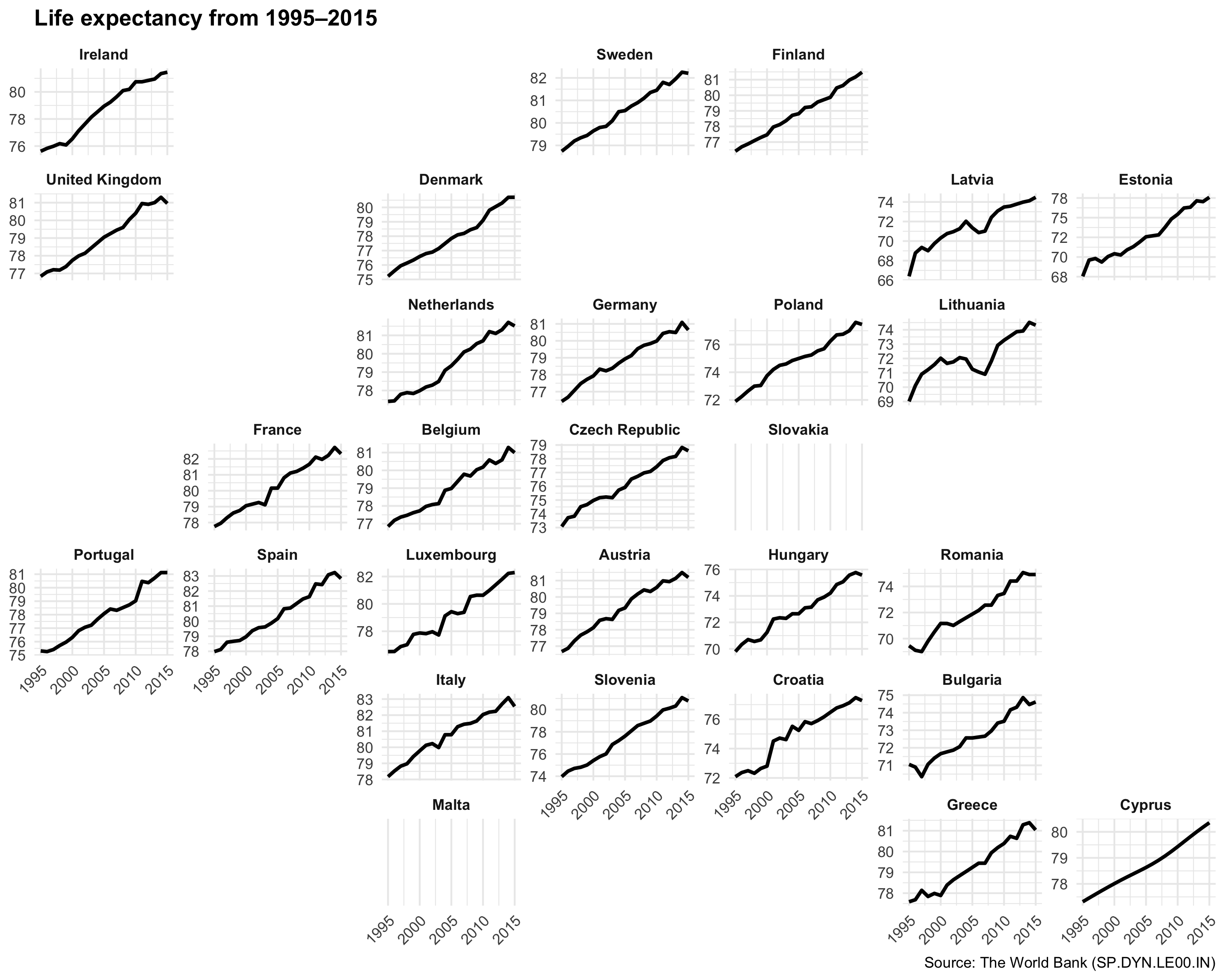
Neat!
Sparklines
Sparklines are just line charts (or bar charts) that are really really small.
india_co2 <- wdi_clean %>%
  filter(country == "India")

plot_india <- ggplot(india_co2, aes(x = year, y = co2_emissions)) +
  geom_line() +
  theme_void()
plot_india
ggsave("india_co2.pdf", plot_india, width = 1, height = 0.15, units = "in")
ggsave("india_co2.png", plot_india, width = 1, height = 0.15, units = "in")
china_co2 <- wdi_clean %>%
  filter(country == "China")

plot_china <- ggplot(china_co2, aes(x = year, y = co2_emissions)) +
  geom_line() +
  theme_void()
plot_china

ggsave("china_co2.pdf", plot_china, width = 1, heighlt = 0.15, units = "in")
ggsave("china_co2.png", plot_china, width = 1, height = 0.15, units = "in")
You can then use those saved tiny plots in your text.
Both India
Slopegraphs
We can make a slopegraph to show changes in GDP per capita between two time periods. We need to first filter our WDI to include only the start and end years (here 1995 and 2015). Then, to make sure that we’re using complete data, we’ll get rid of any country that has missing data for either 1995 or 2015. The group_by(...) %>% filter(...) %>% ungroup() pipeline does this, with the !any(is.na(gdp_per_cap)) test keeping any rows where any of the gdp_per_cap values are not missing for the whole country.
We then add a couple special columns for labels. The paste0() function concatenates strings and variables together, so that paste0("2 + 2 = ", 2 + 2) would show “2 + 2 = 4”. Here we make labels that say either “Country name: $GDP” or “$GDP” depending on the year.
gdp_south_asia <- wdi_clean %>%
  filter(region == "South Asia") %>%
  filter(year %in% c(1995, 2015)) %>%
  # Look at each country individually
  group_by(country) %>%
  # Remove the country if any of its gdp_per_cap values are missing
  filter(!any(is.na(gdp_per_cap))) %>%
  ungroup() %>%
  # Make year a factor
  mutate(year = factor(year)) %>%
  # Make some nice label columns
  # If the year is 1995, format it like "Country name: $GDP". If the year is
  # 2015, format it like "$GDP"
  mutate(label_first = ifelse(year == 1995, paste0(country, ": ", dollar(round(gdp_per_cap))), NA),
         label_last = ifelse(year == 2015, dollar(round(gdp_per_cap, 0)), NA))
With the data filtered like this, we can plot it by mapping year to the x-axis, GDP per capita to the y-axis, and coloring by country. To make the lines go across the two categorical labels in the x-axis (since we made year a factor/category), we need to also specify the group aesthetic.
ggplot(gdp_south_asia, aes(x = year, y = gdp_per_cap, group = country, color = country)) +
  geom_line(size = 1.5)
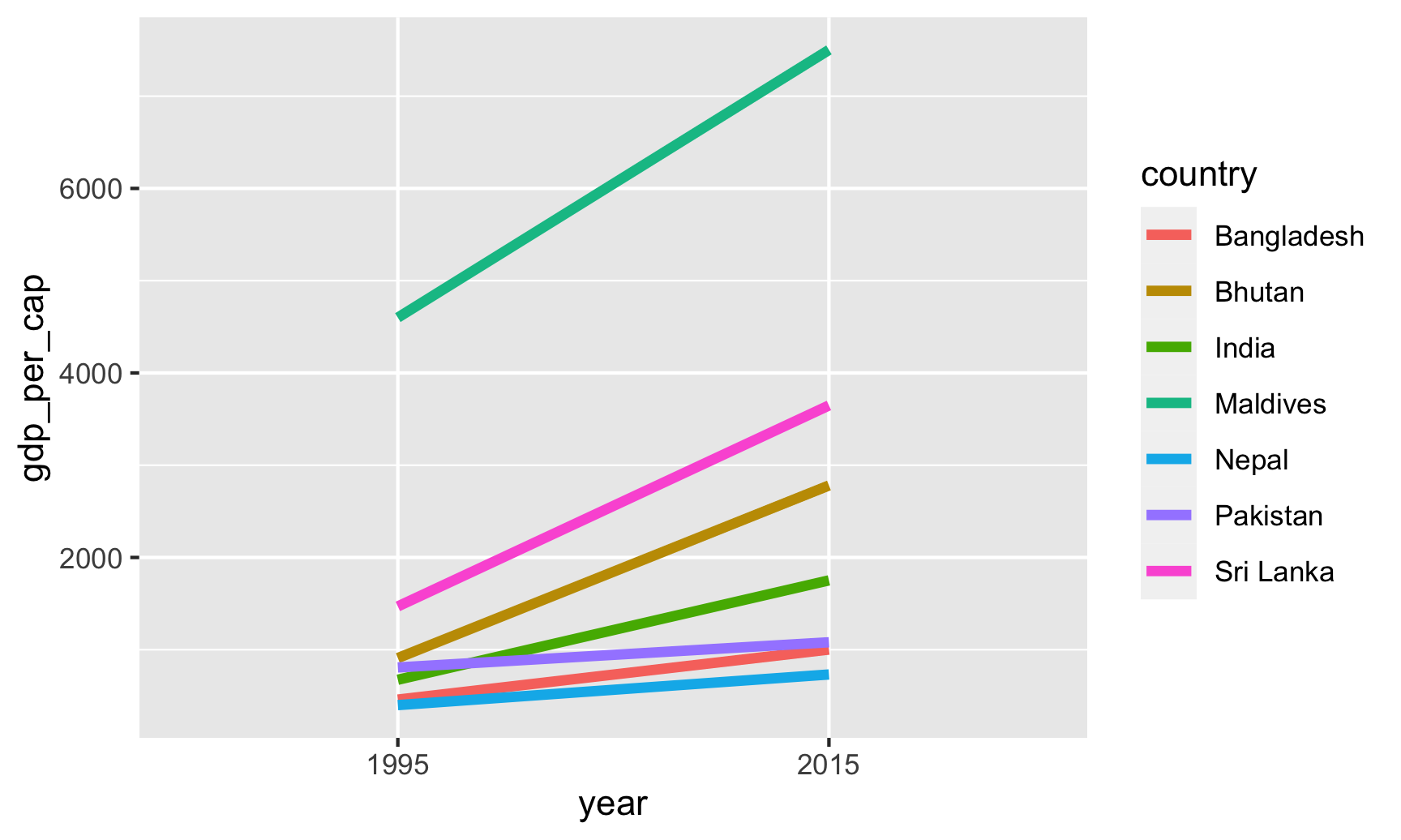
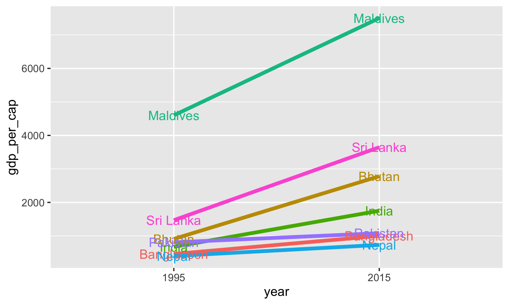
Cool! We’re getting closer. We can definitely see different slopes, but with 7 different colors, it’s hard to see exactly which country is which. Instead, we can directly label each of these lines with geom_text():
ggplot(gdp_south_asia, aes(x = year, y = gdp_per_cap, group = country, color = country)) +
  geom_line(size = 1.5) +
  geom_text(aes(label = country)) +
  guides(color = "none")
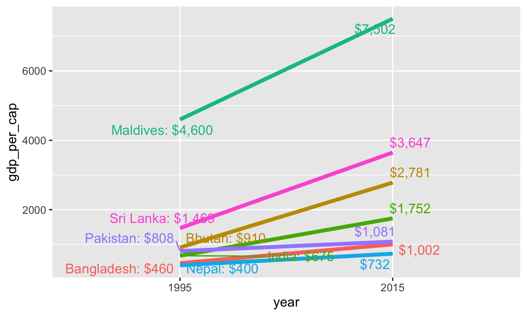
That gets us a little closer, but the country labels are hard to see, and we could include more information, like the actual values. Remember those label_first and label_last columns we made? Let’s use those instead:
ggplot(gdp_south_asia, aes(x = year, y = gdp_per_cap, group = country, color = country)) +
  geom_line(size = 1.5) +
  geom_text(aes(label = label_first)) +
  geom_text(aes(label = label_last)) +
  guides(color = "none")
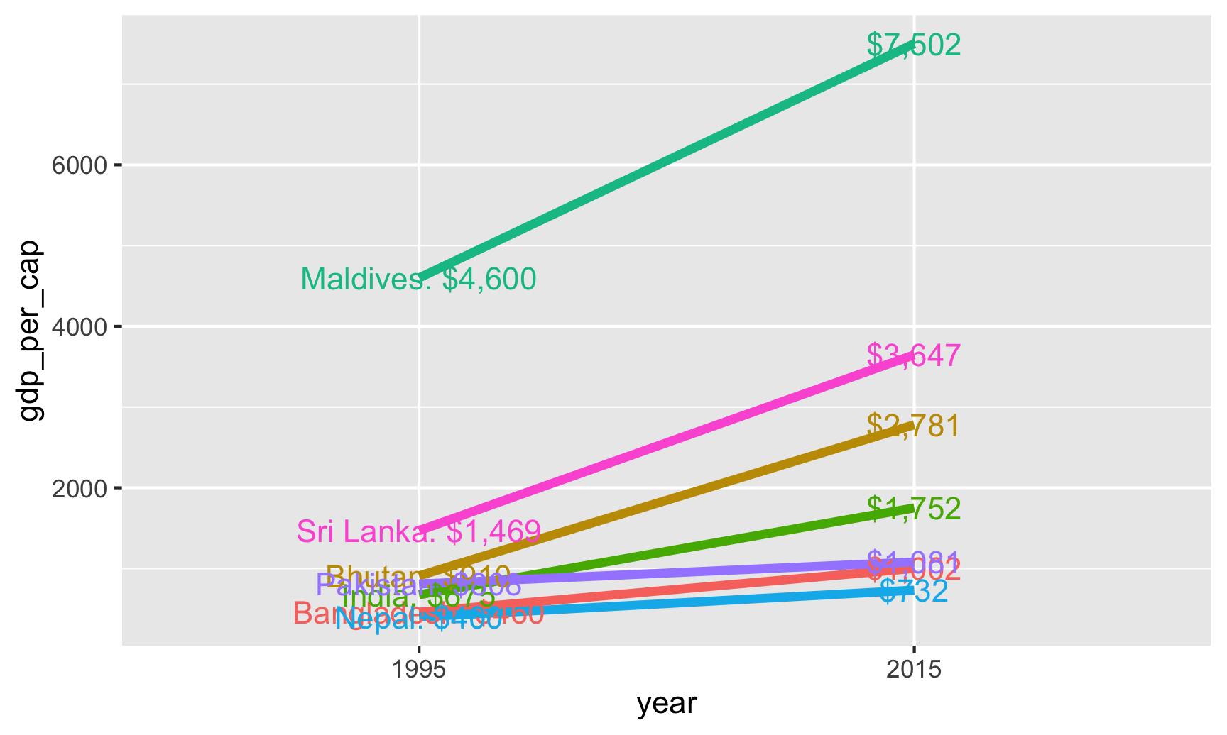
Now we have dollar amounts and country names, but the labels are still overlapping and really hard to read. To fix this, we can make the labels repel away from each other and randomly position in a way that makes them not overlap. The ggrepel package lets us do this with geom_text_repel()
ggplot(gdp_south_asia, aes(x = year, y = gdp_per_cap, group = country, color = country)) +
  geom_line(size = 1.5) +
  geom_text_repel(aes(label = label_first)) +
  geom_text_repel(aes(label = label_last)) +
  guides(color = "none")
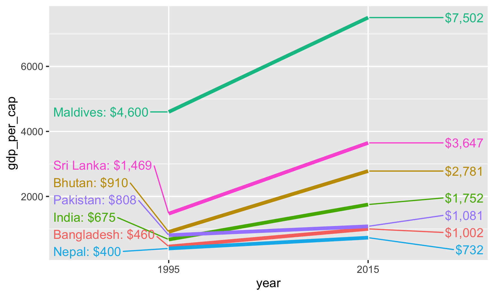
Now none of the labels are on top of each other, but the labels are still on top of the lines. Also, some of the labels moved inward and outward along the x-axis, but they don’t need to do that—they just need to shift up and down. We can force the labels to only move up and down by setting the direction = "y" argument, and we can move all the labels to the left or right with the nudge_x argument. The seed argument makes sure that the random label placement is the same every time we run this. It can be whatever number you want—it just has to be a number.
ggplot(gdp_south_asia, aes(x = year, y = gdp_per_cap, group = country, color = country)) +
  geom_line(size = 1.5) +
  geom_text_repel(aes(label = label_first), direction = "y", nudge_x = -1, seed = 1234) +
  geom_text_repel(aes(label = label_last), direction = "y", nudge_x = 1, seed = 1234) +
  guides(color = "none")
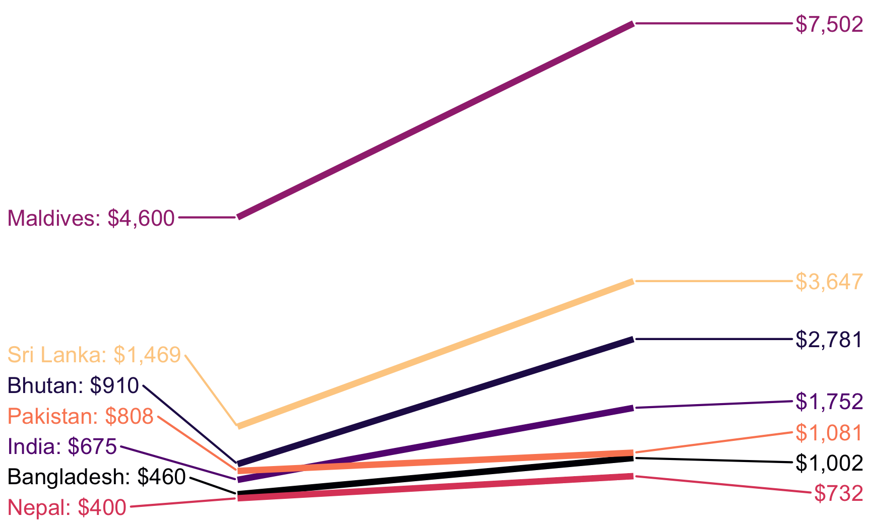
That’s it! Let’s take the theme off completely, change the colors a little, and it should be perfect.
ggplot(gdp_south_asia, aes(x = year, y = gdp_per_cap, group = country, color = country)) +
  geom_line(size = 1.5) +
  geom_text_repel(aes(label = label_first), direction = "y", nudge_x = -1, seed = 1234) +
  geom_text_repel(aes(label = label_last), direction = "y", nudge_x = 1, seed = 1234) +
  guides(color = "none") +
  scale_color_viridis_d(option = "magma", end = 0.9) +
  theme_void()
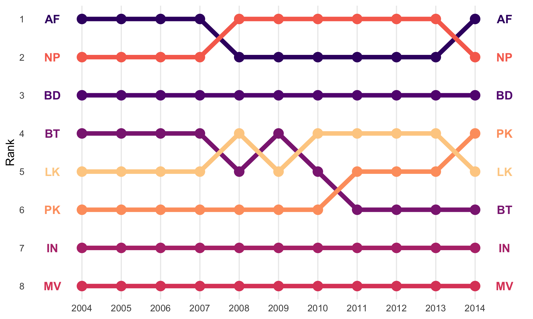
Bump charts
Finally, we can make a bump chart that shows changes in rankings over time. We’ll look at CO2 emissions in South Asia. First we need to calculate a new variable that shows the rank of each country within each year. We can do this if we group by year and then use the rank() function to rank countries by the co2_emissions column.
sa_co2 <- wdi_clean %>%
  filter(region == "South Asia") %>%
  filter(year >= 2004, year < 2015) %>%
  group_by(year) %>%
  mutate(rank = rank(co2_emissions))
We then plot this with points and lines, reversing the y-axis so 1 is at the top:
ggplot(sa_co2, aes(x = year, y = rank, color = country)) +
  geom_line() +
  geom_point() +
  scale_y_reverse(breaks = 1:8)
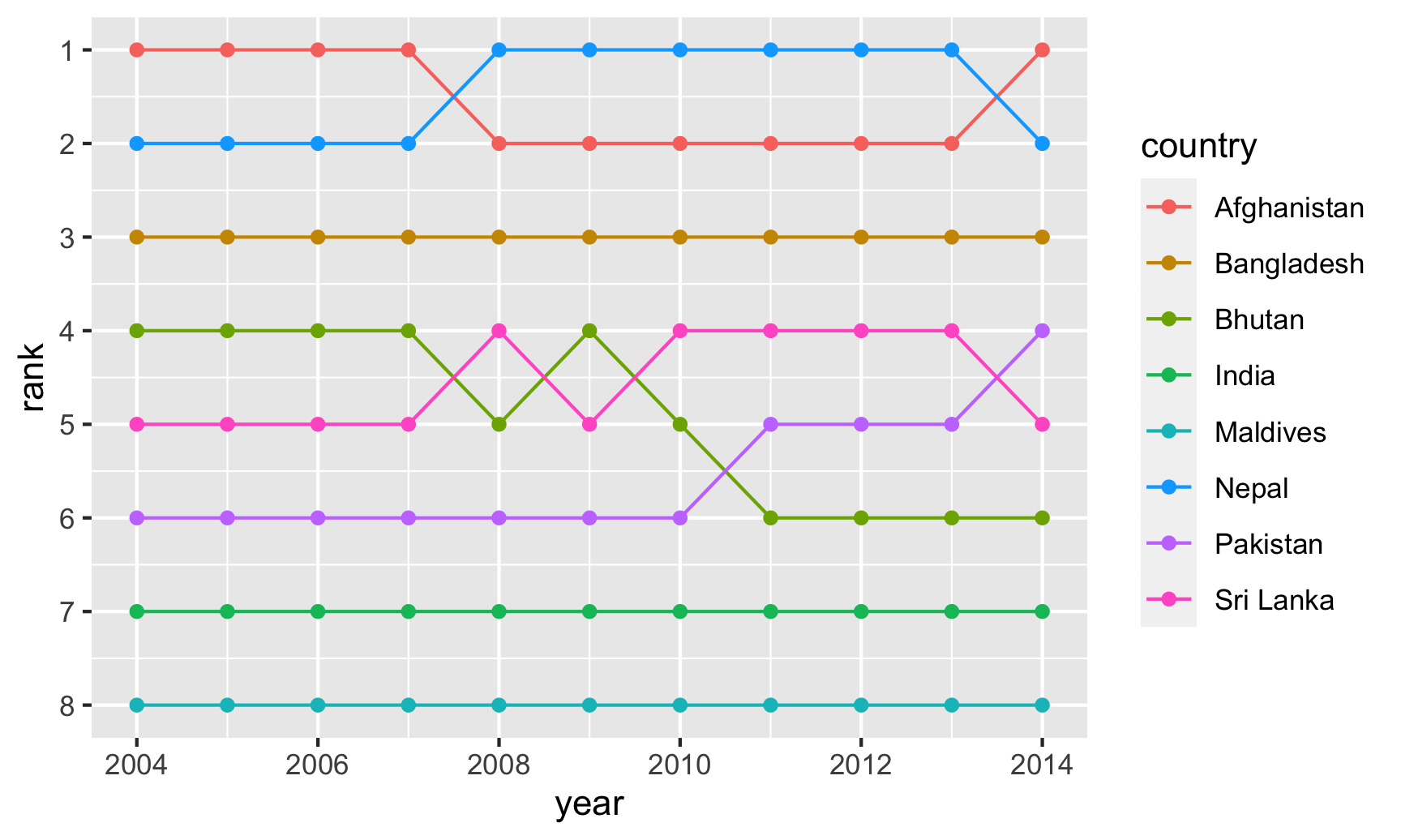
Afghanistan and Nepal switched around for the number 1 spot, while India dropped from 4 to 6, switching places with Pakistan.
As with the slopegraph, there are 8 different colors in the legend and it’s hard to line them all up with the different lines, so we can plot the text directly instead. We’ll use geom_text() again. We don’t need to repel anything, since the text should fit in each row just fine. We need to change the data argument in geom_text() though and filter the data to only include one year, otherwise we’ll get labels on every point, which is excessive. We can also adjust the theme and colors to make it cleaner.
ggplot(sa_co2, aes(x = year, y = rank, color = country)) +
  geom_line(size = 2) +
  geom_point(size = 4) +
  geom_text(data = filter(sa_co2, year == 2004),
            aes(label = iso2c, x = 2003.25),
            fontface = "bold") +
  geom_text(data = filter(sa_co2, year == 2014),
            aes(label = iso2c, x = 2014.75),
            fontface = "bold") +
  guides(color = "none") +
  scale_y_reverse(breaks = 1:8) +
  scale_x_continuous(breaks = 2004:2014) +
  scale_color_viridis_d(option = "magma", begin = 0.2, end = 0.9) +
  labs(x = NULL, y = "Rank") +
  theme_minimal() +
  theme(panel.grid.major.y = element_blank(),
        panel.grid.minor.y = element_blank(),
        panel.grid.minor.x = element_blank())
If you want to be super fancy, you can use flags instead of country codes, but that’s a little more complicated (you need to install the ggflags package. See here for an example.